Computes a suite of diagnostic values for an MLMC estimation problem.
Usage
mlmc.test(
  mlmc_l,
  N,
  L,
  N0,
  eps.v,
  Lmin,
  Lmax,
  alpha = NA,
  beta = NA,
  gamma = NA,
  parallel = NA,
  silent = FALSE,
  ...
)
Arguments
- mlmc_l
a user supplied function which provides the estimate for level \(l\). It must take at least two arguments, the first is the level number to be simulated and the second the number of paths. Additional arguments can be taken if desired: all additional
...arguments to this function are forwarded to the user definedmlmc_lfunction.The user supplied function should return a named list containing one element named
sumsand second namedcost, where:sumsis a vector of length six \(\left(\sum Y_i, \sum Y_i^2, \sum Y_i^3, \sum Y_i^4, \sum X_i, \sum X_i^2\right)\) where \(Y_i\) are iid simulations with expectation \(E[P_0]\) when \(l=0\) and expectation \(E[P_l-P_{l-1}]\) when \(l>0\), and \(X_i\) are iid simulations with expectation \(E[P_l]\). Note that this differs from the main
mlmc()driver, which only requires the first two of these elements in order to calculate the estimate. The remaining elements are required bymlmc.test()since they are used for convergence tests, kurtosis, and telescoping sum checks.costis a scalar with the total cost of the paths simulated. For example, in the financial options samplers included in this package, this is calculated as \(NM^l\), where \(N\) is the number of paths requested in the call to the user function
mlmc_l, \(M\) is the refinement cost factor (\(M=2\) formcqmc06_l()and \(M=4\) foropre_l()), and \(l\) is the level being sampled.
See the function (and source code of)
opre_l()andmcqmc06_l()in this package for an example of user supplied level samplers.- N
number of samples to use in convergence tests, kurtosis, telescoping sum check.
- L
number of levels to use in convergence tests, kurtosis, telescoping sum check.
- N0
initial number of samples which are used for the first 3 levels and for any subsequent levels which are automatically added in the complexity tests. Must be \(> 0\).
- eps.v
a vector of one or more target accuracies for the complexity tests. Must all be \(> 0\).
- Lmin
the minimum level of refinement for complexity tests. Must be \(\ge 2\).
- Lmax
the maximum level of refinement for complexity tests. Must be \(\ge\)
Lmin.- alpha
the weak error, \(O(2^{-\alpha l})\). Must be \(> 0\) if specified. If
NAthenalphawill be estimated.- beta
the variance, \(O(2^{-\beta l})\). Must be \(> 0\) if specified. If
NAthenbetawill be estimated.- gamma
the sample cost, \(O(2^{\gamma l})\). Must be \(> 0\) if specified. If
NAthengammawill be estimated.- parallel
if an integer is supplied, R will fork
parallelparallel processes. This is done for the convergence tests section by splitting theNsamples as evenly as possible across cores when sampling each level. This is also done for the MLMC complexity tests by passing theparallelargument on to themlmc()driver when targeting each accuracy level ineps.- silent
set to TRUE to supress running output (identical output can still be printed by printing the return result)
- ...
additional arguments which are passed on when the user supplied
mlmc_lfunction is called
Value
An mlmc.test object which contains all the computed diagnostic values.
This object can be printed or plotted (see plot.mlmc.test).
Details
See one of the example level sampler functions (e.g. opre_l()) for example usage.
This function is based on GPL-2 'Matlab' code by Mike Giles.
Author
Louis Aslett <louis.aslett@durham.ac.uk>
Mike Giles <Mike.Giles@maths.ox.ac.uk>
Tigran Nagapetyan <nagapetyan@stats.ox.ac.uk>
Examples
# \donttest{
# Example calls with realistic arguments
# Financial options using an Euler-Maruyama discretisation
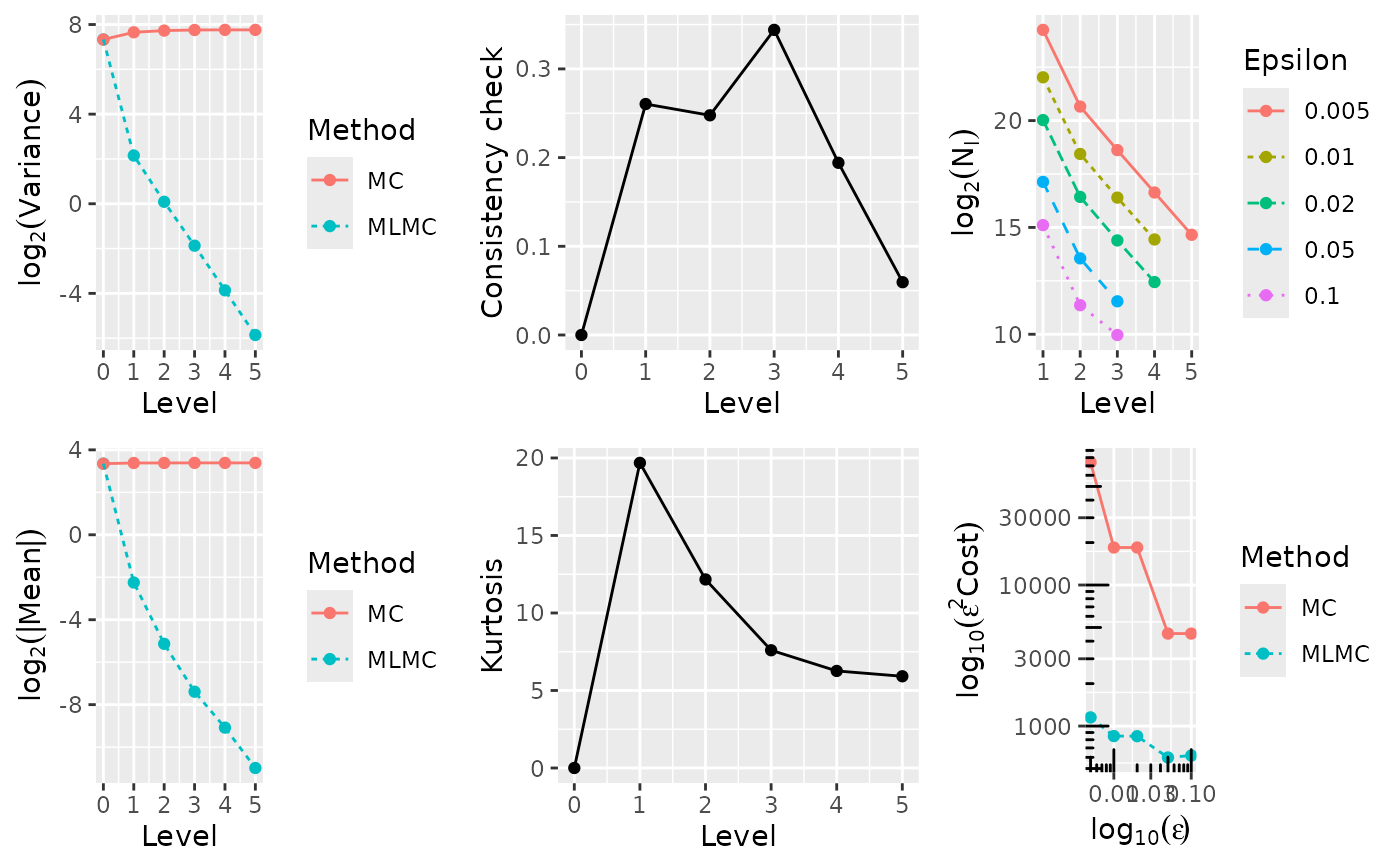
tst <- mlmc.test(opre_l, N = 2000000,
L = 5, N0 = 1000,
eps.v = c(0.005, 0.01, 0.02, 0.05, 0.1),
Lmin = 2, Lmax = 6,
option = 1)
#>
#> **********************************************************
#> *** Convergence tests, kurtosis, telescoping sum check ***
#> *** using N = 2e+06 samples ***
#> **********************************************************
#>
#> l ave(Pf-Pc) ave(Pf) var(Pf-Pc) var(Pf) kurtosis check cost
#> ---------------------------------------------------------------------------------------
#> 0 1.0204e+01 1.0204e+01 1.6112e+02 1.6112e+02 0.0000e+00 0.0000e+00 1.0000e+00
#> 1 2.0823e-01 1.0408e+01 4.4300e+00 2.0069e+02 1.9950e+01 7.0028e-02 4.0000e+00
#> 2 2.9454e-02 1.0442e+01 1.0630e+00 2.1246e+02 1.1884e+01 7.2635e-02 1.6000e+01
#> 3 5.5716e-03 1.0445e+01 2.7285e-01 2.1571e+02 7.5682e+00 3.8539e-02 6.4000e+01
#> 4 9.9419e-04 1.0451e+01 6.8728e-02 2.1639e+02 6.1931e+00 8.7064e-02 2.5600e+02
#> 5 3.3227e-04 1.0454e+01 1.7298e-02 2.1673e+02 5.9412e+00 4.6263e-02 1.0240e+03
#>
#> ******************************************************
#> *** Linear regression estimates of MLMC parameters ***
#> ******************************************************
#>
#> alpha = 2.347198 (exponent for MLMC weak convergence)
#> beta = 1.995233 (exponent for MLMC variance)
#> gamma = 2.000000 (exponent for MLMC cost)
#>
#> *****************************
#> *** MLMC complexity tests ***
#> *****************************
#>
#> eps value mlmc_cost std_cost savings N_l
#> -----------------------------------------------------------
#> 0.0050 1.0449e+01 3.385e+07 7.363e+08 21.75 17059567 1416680 345867 87369
#> 0.0100 1.0442e+01 8.466e+06 1.841e+08 21.74 4261790 353226 86554 21977
#> 0.0200 1.0440e+01 2.139e+06 4.602e+07 21.51 1071580 89891 21660 5646
#> 0.0500 1.0477e+01 2.388e+05 1.813e+06 7.59 142815 11837 3042
#> 0.1000 1.0486e+01 6.828e+04 4.533e+05 6.64 38083 3549 1000
#>
tst
#>
#> **********************************************************
#> *** Convergence tests, kurtosis, telescoping sum check ***
#> *** using N = 2e+06 samples ***
#> **********************************************************
#>
#> l ave(Pf-Pc) ave(Pf) var(Pf-Pc) var(Pf) kurtosis check cost
#> ---------------------------------------------------------------------------------------
#> 0 1.0204e+01 1.0204e+01 1.6112e+02 1.6112e+02 0.0000e+00 0.0000e+00 1.0000e+00
#> 1 2.0823e-01 1.0408e+01 4.4300e+00 2.0069e+02 1.9950e+01 7.0028e-02 4.0000e+00
#> 2 2.9454e-02 1.0442e+01 1.0630e+00 2.1246e+02 1.1884e+01 7.2635e-02 1.6000e+01
#> 3 5.5716e-03 1.0445e+01 2.7285e-01 2.1571e+02 7.5682e+00 3.8539e-02 6.4000e+01
#> 4 9.9419e-04 1.0451e+01 6.8728e-02 2.1639e+02 6.1931e+00 8.7064e-02 2.5600e+02
#> 5 3.3227e-04 1.0454e+01 1.7298e-02 2.1673e+02 5.9412e+00 4.6263e-02 1.0240e+03
#>
#> ******************************************************
#> *** Linear regression estimates of MLMC parameters ***
#> ******************************************************
#>
#> alpha = 2.347198 (exponent for MLMC weak convergence)
#> beta = 1.995233 (exponent for MLMC variance)
#> gamma = 2.000000 (exponent for MLMC cost)
#>
#> *****************************
#> *** MLMC complexity tests ***
#> *****************************
#>
#> eps value mlmc_cost std_cost savings N_l
#> -----------------------------------------------------------
#> 0.0050 1.0449e+01 3.385e+07 7.363e+08 21.75 17059567 1416680 345867 87369
#> 0.0100 1.0442e+01 8.466e+06 1.841e+08 21.74 4261790 353226 86554 21977
#> 0.0200 1.0440e+01 2.139e+06 4.602e+07 21.51 1071580 89891 21660 5646
#> 0.0500 1.0477e+01 2.388e+05 1.813e+06 7.59 142815 11837 3042
#> 0.1000 1.0486e+01 6.828e+04 4.533e+05 6.64 38083 3549 1000
#>
plot(tst)
 # Financial options using a Milstein discretisation
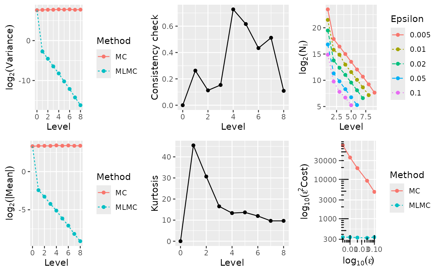
tst <- mlmc.test(mcqmc06_l, N = 20000,
L = 8, N0 = 200,
eps.v = c(0.005, 0.01, 0.02, 0.05, 0.1),
Lmin = 2, Lmax = 10,
option = 1)
#>
#> **********************************************************
#> *** Convergence tests, kurtosis, telescoping sum check ***
#> *** using N = 20000 samples ***
#> **********************************************************
#>
#> l ave(Pf-Pc) ave(Pf) var(Pf-Pc) var(Pf) kurtosis check cost
#> ---------------------------------------------------------------------------------------
#> 0 9.9678e+00 9.9678e+00 1.9425e+02 1.9425e+02 0.0000e+00 0.0000e+00 1.0000e+00
#> 1 1.8854e-01 1.0433e+01 1.6048e-01 2.0933e+02 6.2192e+01 4.5298e-01 2.0000e+00
#> 2 1.0292e-01 1.0325e+01 4.2479e-02 2.0797e+02 3.6113e+01 3.4222e-01 4.0000e+00
#> 3 5.3887e-02 1.0291e+01 1.1557e-02 2.0988e+02 2.1362e+01 1.4261e-01 8.0000e+00
#> 4 2.8099e-02 1.0457e+01 3.2718e-03 2.1643e+02 1.4462e+01 2.2270e-01 1.6000e+01
#> 5 1.4336e-02 1.0512e+01 8.5604e-04 2.2097e+02 1.4364e+01 6.4064e-02 3.2000e+01
#> 6 7.2362e-03 1.0575e+01 2.1685e-04 2.2159e+02 1.0578e+01 8.8081e-02 6.4000e+01
#> 7 3.4321e-03 1.0385e+01 5.1794e-05 2.1177e+02 1.0726e+01 3.0914e-01 1.2800e+02
#> 8 1.8311e-03 1.0661e+01 1.3848e-05 2.2126e+02 9.7964e+00 4.3982e-01 2.5600e+02
#>
#> ******************************************************
#> *** Linear regression estimates of MLMC parameters ***
#> ******************************************************
#>
#> alpha = 0.964223 (exponent for MLMC weak convergence)
#> beta = 1.929095 (exponent for MLMC variance)
#> gamma = 1.000000 (exponent for MLMC cost)
#>
#> *****************************
#> *** MLMC complexity tests ***
#> *****************************
#>
#> eps value mlmc_cost std_cost savings N_l
#> -----------------------------------------------------------
#> 0.0050 1.0453e+01 1.356e+07 3.021e+09 222.85 11904499 231846 88907 33376 11796 4481 1610 578 219
#> 0.0100 1.0454e+01 3.367e+06 3.614e+08 107.34 2975084 58567 21189 8155 2857 1096 401 145
#> 0.0200 1.0468e+01 8.360e+05 4.727e+07 56.55 739677 14415 5783 2098 751 274 106
#> 0.0500 1.0513e+01 1.325e+05 3.771e+06 28.47 118210 2121 837 327 148 53
#> 0.1000 1.0373e+01 3.285e+04 4.617e+05 14.06 29521 494 265 92 34
#>
tst
#>
#> **********************************************************
#> *** Convergence tests, kurtosis, telescoping sum check ***
#> *** using N = 20000 samples ***
#> **********************************************************
#>
#> l ave(Pf-Pc) ave(Pf) var(Pf-Pc) var(Pf) kurtosis check cost
#> ---------------------------------------------------------------------------------------
#> 0 9.9678e+00 9.9678e+00 1.9425e+02 1.9425e+02 0.0000e+00 0.0000e+00 1.0000e+00
#> 1 1.8854e-01 1.0433e+01 1.6048e-01 2.0933e+02 6.2192e+01 4.5298e-01 2.0000e+00
#> 2 1.0292e-01 1.0325e+01 4.2479e-02 2.0797e+02 3.6113e+01 3.4222e-01 4.0000e+00
#> 3 5.3887e-02 1.0291e+01 1.1557e-02 2.0988e+02 2.1362e+01 1.4261e-01 8.0000e+00
#> 4 2.8099e-02 1.0457e+01 3.2718e-03 2.1643e+02 1.4462e+01 2.2270e-01 1.6000e+01
#> 5 1.4336e-02 1.0512e+01 8.5604e-04 2.2097e+02 1.4364e+01 6.4064e-02 3.2000e+01
#> 6 7.2362e-03 1.0575e+01 2.1685e-04 2.2159e+02 1.0578e+01 8.8081e-02 6.4000e+01
#> 7 3.4321e-03 1.0385e+01 5.1794e-05 2.1177e+02 1.0726e+01 3.0914e-01 1.2800e+02
#> 8 1.8311e-03 1.0661e+01 1.3848e-05 2.2126e+02 9.7964e+00 4.3982e-01 2.5600e+02
#>
#> ******************************************************
#> *** Linear regression estimates of MLMC parameters ***
#> ******************************************************
#>
#> alpha = 0.964223 (exponent for MLMC weak convergence)
#> beta = 1.929095 (exponent for MLMC variance)
#> gamma = 1.000000 (exponent for MLMC cost)
#>
#> *****************************
#> *** MLMC complexity tests ***
#> *****************************
#>
#> eps value mlmc_cost std_cost savings N_l
#> -----------------------------------------------------------
#> 0.0050 1.0453e+01 1.356e+07 3.021e+09 222.85 11904499 231846 88907 33376 11796 4481 1610 578 219
#> 0.0100 1.0454e+01 3.367e+06 3.614e+08 107.34 2975084 58567 21189 8155 2857 1096 401 145
#> 0.0200 1.0468e+01 8.360e+05 4.727e+07 56.55 739677 14415 5783 2098 751 274 106
#> 0.0500 1.0513e+01 1.325e+05 3.771e+06 28.47 118210 2121 837 327 148 53
#> 0.1000 1.0373e+01 3.285e+04 4.617e+05 14.06 29521 494 265 92 34
#>
plot(tst)
# Financial options using a Milstein discretisation
tst <- mlmc.test(mcqmc06_l, N = 20000,
L = 8, N0 = 200,
eps.v = c(0.005, 0.01, 0.02, 0.05, 0.1),
Lmin = 2, Lmax = 10,
option = 1)
#>
#> **********************************************************
#> *** Convergence tests, kurtosis, telescoping sum check ***
#> *** using N = 20000 samples ***
#> **********************************************************
#>
#> l ave(Pf-Pc) ave(Pf) var(Pf-Pc) var(Pf) kurtosis check cost
#> ---------------------------------------------------------------------------------------
#> 0 9.9678e+00 9.9678e+00 1.9425e+02 1.9425e+02 0.0000e+00 0.0000e+00 1.0000e+00
#> 1 1.8854e-01 1.0433e+01 1.6048e-01 2.0933e+02 6.2192e+01 4.5298e-01 2.0000e+00
#> 2 1.0292e-01 1.0325e+01 4.2479e-02 2.0797e+02 3.6113e+01 3.4222e-01 4.0000e+00
#> 3 5.3887e-02 1.0291e+01 1.1557e-02 2.0988e+02 2.1362e+01 1.4261e-01 8.0000e+00
#> 4 2.8099e-02 1.0457e+01 3.2718e-03 2.1643e+02 1.4462e+01 2.2270e-01 1.6000e+01
#> 5 1.4336e-02 1.0512e+01 8.5604e-04 2.2097e+02 1.4364e+01 6.4064e-02 3.2000e+01
#> 6 7.2362e-03 1.0575e+01 2.1685e-04 2.2159e+02 1.0578e+01 8.8081e-02 6.4000e+01
#> 7 3.4321e-03 1.0385e+01 5.1794e-05 2.1177e+02 1.0726e+01 3.0914e-01 1.2800e+02
#> 8 1.8311e-03 1.0661e+01 1.3848e-05 2.2126e+02 9.7964e+00 4.3982e-01 2.5600e+02
#>
#> ******************************************************
#> *** Linear regression estimates of MLMC parameters ***
#> ******************************************************
#>
#> alpha = 0.964223 (exponent for MLMC weak convergence)
#> beta = 1.929095 (exponent for MLMC variance)
#> gamma = 1.000000 (exponent for MLMC cost)
#>
#> *****************************
#> *** MLMC complexity tests ***
#> *****************************
#>
#> eps value mlmc_cost std_cost savings N_l
#> -----------------------------------------------------------
#> 0.0050 1.0453e+01 1.356e+07 3.021e+09 222.85 11904499 231846 88907 33376 11796 4481 1610 578 219
#> 0.0100 1.0454e+01 3.367e+06 3.614e+08 107.34 2975084 58567 21189 8155 2857 1096 401 145
#> 0.0200 1.0468e+01 8.360e+05 4.727e+07 56.55 739677 14415 5783 2098 751 274 106
#> 0.0500 1.0513e+01 1.325e+05 3.771e+06 28.47 118210 2121 837 327 148 53
#> 0.1000 1.0373e+01 3.285e+04 4.617e+05 14.06 29521 494 265 92 34
#>
tst
#>
#> **********************************************************
#> *** Convergence tests, kurtosis, telescoping sum check ***
#> *** using N = 20000 samples ***
#> **********************************************************
#>
#> l ave(Pf-Pc) ave(Pf) var(Pf-Pc) var(Pf) kurtosis check cost
#> ---------------------------------------------------------------------------------------
#> 0 9.9678e+00 9.9678e+00 1.9425e+02 1.9425e+02 0.0000e+00 0.0000e+00 1.0000e+00
#> 1 1.8854e-01 1.0433e+01 1.6048e-01 2.0933e+02 6.2192e+01 4.5298e-01 2.0000e+00
#> 2 1.0292e-01 1.0325e+01 4.2479e-02 2.0797e+02 3.6113e+01 3.4222e-01 4.0000e+00
#> 3 5.3887e-02 1.0291e+01 1.1557e-02 2.0988e+02 2.1362e+01 1.4261e-01 8.0000e+00
#> 4 2.8099e-02 1.0457e+01 3.2718e-03 2.1643e+02 1.4462e+01 2.2270e-01 1.6000e+01
#> 5 1.4336e-02 1.0512e+01 8.5604e-04 2.2097e+02 1.4364e+01 6.4064e-02 3.2000e+01
#> 6 7.2362e-03 1.0575e+01 2.1685e-04 2.2159e+02 1.0578e+01 8.8081e-02 6.4000e+01
#> 7 3.4321e-03 1.0385e+01 5.1794e-05 2.1177e+02 1.0726e+01 3.0914e-01 1.2800e+02
#> 8 1.8311e-03 1.0661e+01 1.3848e-05 2.2126e+02 9.7964e+00 4.3982e-01 2.5600e+02
#>
#> ******************************************************
#> *** Linear regression estimates of MLMC parameters ***
#> ******************************************************
#>
#> alpha = 0.964223 (exponent for MLMC weak convergence)
#> beta = 1.929095 (exponent for MLMC variance)
#> gamma = 1.000000 (exponent for MLMC cost)
#>
#> *****************************
#> *** MLMC complexity tests ***
#> *****************************
#>
#> eps value mlmc_cost std_cost savings N_l
#> -----------------------------------------------------------
#> 0.0050 1.0453e+01 1.356e+07 3.021e+09 222.85 11904499 231846 88907 33376 11796 4481 1610 578 219
#> 0.0100 1.0454e+01 3.367e+06 3.614e+08 107.34 2975084 58567 21189 8155 2857 1096 401 145
#> 0.0200 1.0468e+01 8.360e+05 4.727e+07 56.55 739677 14415 5783 2098 751 274 106
#> 0.0500 1.0513e+01 1.325e+05 3.771e+06 28.47 118210 2121 837 327 148 53
#> 0.1000 1.0373e+01 3.285e+04 4.617e+05 14.06 29521 494 265 92 34
#>
plot(tst)
 # }
# Toy versions for CRAN tests
tst <- mlmc.test(opre_l, N = 10000,
L = 5, N0 = 1000,
eps.v = c(0.025, 0.1),
Lmin = 2, Lmax = 6,
option = 1)
#>
#> **********************************************************
#> *** Convergence tests, kurtosis, telescoping sum check ***
#> *** using N = 10000 samples ***
#> **********************************************************
#>
#> l ave(Pf-Pc) ave(Pf) var(Pf-Pc) var(Pf) kurtosis check cost
#> ---------------------------------------------------------------------------------------
#> 0 1.0316e+01 1.0316e+01 1.6448e+02 1.6448e+02 0.0000e+00 0.0000e+00 1.0000e+00
#> 1 2.1482e-01 1.0467e+01 4.3915e+00 2.0111e+02 1.6197e+01 7.3118e-02 4.0000e+00
#> 2 2.2952e-02 1.0371e+01 1.0275e+00 2.1114e+02 1.0880e+01 1.3344e-01 1.6000e+01
#> 3 1.0372e-03 1.0829e+01 2.7891e-01 2.1710e+02 7.2369e+00 5.1159e-01 6.4000e+01
#> 4 -1.6469e-03 1.0471e+01 6.8008e-02 2.1737e+02 6.2140e+00 4.0006e-01 2.5600e+02
#> 5 1.0342e-03 1.0710e+01 1.7836e-02 2.2047e+02 5.8653e+00 2.6667e-01 1.0240e+03
#>
#> ******************************************************
#> *** Linear regression estimates of MLMC parameters ***
#> ******************************************************
#>
#> alpha = 1.919781 (exponent for MLMC weak convergence)
#> beta = 1.980492 (exponent for MLMC variance)
#> gamma = 2.000000 (exponent for MLMC cost)
#>
#> *****************************
#> *** MLMC complexity tests ***
#> *****************************
#>
#> eps value mlmc_cost std_cost savings N_l
#> -----------------------------------------------------------
#> 0.0250 1.0452e+01 1.356e+06 2.964e+07 21.85 682589 56683 13474 3618
#> 0.1000 1.0601e+01 6.374e+04 4.504e+05 7.07 35752 2998 1000
#>
tst <- mlmc.test(mcqmc06_l, N = 10000,
L = 8, N0 = 1000,
eps.v = c(0.025, 0.1),
Lmin = 2, Lmax = 10,
option = 1)
#>
#> **********************************************************
#> *** Convergence tests, kurtosis, telescoping sum check ***
#> *** using N = 10000 samples ***
#> **********************************************************
#>
#> l ave(Pf-Pc) ave(Pf) var(Pf-Pc) var(Pf) kurtosis check cost
#> ---------------------------------------------------------------------------------------
#> 0 9.8527e+00 9.8527e+00 1.8501e+02 1.8501e+02 0.0000e+00 0.0000e+00 1.0000e+00
#> 1 1.8546e-01 1.0287e+01 1.5271e-01 2.0787e+02 3.8494e+01 2.9197e-01 2.0000e+00
#> 2 1.0362e-01 1.0340e+01 4.3872e-02 2.1727e+02 2.6792e+01 5.7917e-02 4.0000e+00
#> 3 5.3614e-02 1.0274e+01 1.1840e-02 2.1559e+02 2.0003e+01 1.3504e-01 8.0000e+00
#> 4 2.8140e-02 1.0473e+01 3.1931e-03 2.1203e+02 1.5111e+01 1.9534e-01 1.6000e+01
#> 5 1.4078e-02 1.0459e+01 8.6198e-04 2.1849e+02 1.3218e+01 3.2377e-02 3.2000e+01
#> 6 7.1770e-03 1.0530e+01 2.1348e-04 2.1570e+02 1.1255e+01 7.2584e-02 6.4000e+01
#> 7 3.5359e-03 1.0378e+01 5.2355e-05 2.1813e+02 9.7525e+00 1.7680e-01 1.2800e+02
#> 8 1.7662e-03 1.0451e+01 1.3059e-05 2.1269e+02 1.0266e+01 8.1112e-02 2.5600e+02
#>
#> ******************************************************
#> *** Linear regression estimates of MLMC parameters ***
#> ******************************************************
#>
#> alpha = 0.965102 (exponent for MLMC weak convergence)
#> beta = 1.933541 (exponent for MLMC variance)
#> gamma = 1.000000 (exponent for MLMC cost)
#>
#> *****************************
#> *** MLMC complexity tests ***
#> *****************************
#>
#> eps value mlmc_cost std_cost savings N_l
#> -----------------------------------------------------------
#> 0.0250 1.0440e+01 5.297e+05 2.945e+07 55.60 471075 8710 3220 1233 516 186 66
#> 0.1000 1.0569e+01 3.704e+04 4.523e+05 12.21 29599 1000 1000 104 38
#>
# }
# Toy versions for CRAN tests
tst <- mlmc.test(opre_l, N = 10000,
L = 5, N0 = 1000,
eps.v = c(0.025, 0.1),
Lmin = 2, Lmax = 6,
option = 1)
#>
#> **********************************************************
#> *** Convergence tests, kurtosis, telescoping sum check ***
#> *** using N = 10000 samples ***
#> **********************************************************
#>
#> l ave(Pf-Pc) ave(Pf) var(Pf-Pc) var(Pf) kurtosis check cost
#> ---------------------------------------------------------------------------------------
#> 0 1.0316e+01 1.0316e+01 1.6448e+02 1.6448e+02 0.0000e+00 0.0000e+00 1.0000e+00
#> 1 2.1482e-01 1.0467e+01 4.3915e+00 2.0111e+02 1.6197e+01 7.3118e-02 4.0000e+00
#> 2 2.2952e-02 1.0371e+01 1.0275e+00 2.1114e+02 1.0880e+01 1.3344e-01 1.6000e+01
#> 3 1.0372e-03 1.0829e+01 2.7891e-01 2.1710e+02 7.2369e+00 5.1159e-01 6.4000e+01
#> 4 -1.6469e-03 1.0471e+01 6.8008e-02 2.1737e+02 6.2140e+00 4.0006e-01 2.5600e+02
#> 5 1.0342e-03 1.0710e+01 1.7836e-02 2.2047e+02 5.8653e+00 2.6667e-01 1.0240e+03
#>
#> ******************************************************
#> *** Linear regression estimates of MLMC parameters ***
#> ******************************************************
#>
#> alpha = 1.919781 (exponent for MLMC weak convergence)
#> beta = 1.980492 (exponent for MLMC variance)
#> gamma = 2.000000 (exponent for MLMC cost)
#>
#> *****************************
#> *** MLMC complexity tests ***
#> *****************************
#>
#> eps value mlmc_cost std_cost savings N_l
#> -----------------------------------------------------------
#> 0.0250 1.0452e+01 1.356e+06 2.964e+07 21.85 682589 56683 13474 3618
#> 0.1000 1.0601e+01 6.374e+04 4.504e+05 7.07 35752 2998 1000
#>
tst <- mlmc.test(mcqmc06_l, N = 10000,
L = 8, N0 = 1000,
eps.v = c(0.025, 0.1),
Lmin = 2, Lmax = 10,
option = 1)
#>
#> **********************************************************
#> *** Convergence tests, kurtosis, telescoping sum check ***
#> *** using N = 10000 samples ***
#> **********************************************************
#>
#> l ave(Pf-Pc) ave(Pf) var(Pf-Pc) var(Pf) kurtosis check cost
#> ---------------------------------------------------------------------------------------
#> 0 9.8527e+00 9.8527e+00 1.8501e+02 1.8501e+02 0.0000e+00 0.0000e+00 1.0000e+00
#> 1 1.8546e-01 1.0287e+01 1.5271e-01 2.0787e+02 3.8494e+01 2.9197e-01 2.0000e+00
#> 2 1.0362e-01 1.0340e+01 4.3872e-02 2.1727e+02 2.6792e+01 5.7917e-02 4.0000e+00
#> 3 5.3614e-02 1.0274e+01 1.1840e-02 2.1559e+02 2.0003e+01 1.3504e-01 8.0000e+00
#> 4 2.8140e-02 1.0473e+01 3.1931e-03 2.1203e+02 1.5111e+01 1.9534e-01 1.6000e+01
#> 5 1.4078e-02 1.0459e+01 8.6198e-04 2.1849e+02 1.3218e+01 3.2377e-02 3.2000e+01
#> 6 7.1770e-03 1.0530e+01 2.1348e-04 2.1570e+02 1.1255e+01 7.2584e-02 6.4000e+01
#> 7 3.5359e-03 1.0378e+01 5.2355e-05 2.1813e+02 9.7525e+00 1.7680e-01 1.2800e+02
#> 8 1.7662e-03 1.0451e+01 1.3059e-05 2.1269e+02 1.0266e+01 8.1112e-02 2.5600e+02
#>
#> ******************************************************
#> *** Linear regression estimates of MLMC parameters ***
#> ******************************************************
#>
#> alpha = 0.965102 (exponent for MLMC weak convergence)
#> beta = 1.933541 (exponent for MLMC variance)
#> gamma = 1.000000 (exponent for MLMC cost)
#>
#> *****************************
#> *** MLMC complexity tests ***
#> *****************************
#>
#> eps value mlmc_cost std_cost savings N_l
#> -----------------------------------------------------------
#> 0.0250 1.0440e+01 5.297e+05 2.945e+07 55.60 471075 8710 3220 1233 516 186 66
#> 0.1000 1.0569e+01 3.704e+04 4.523e+05 12.21 29599 1000 1000 104 38
#>