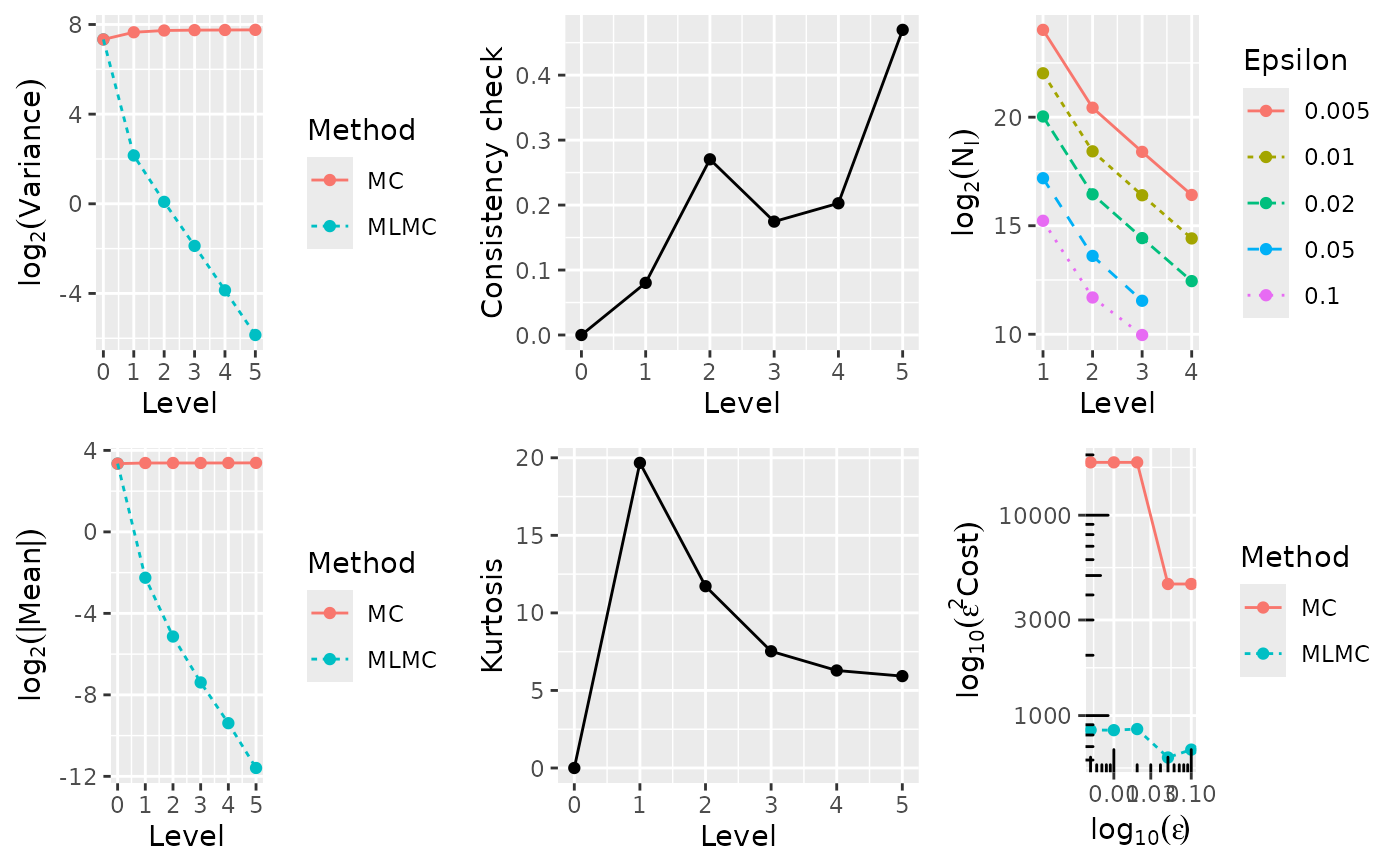
Produces diagnostic plots on the result of an mlmc.test function call.
Usage
# S3 method for class 'mlmc.test'
plot(x, which = "all", cols = NA, ...)
Arguments
- x
an
mlmc.testobject as produced by a call to themlmc.testfunction.- which
a vector of strings specifying which plots to produce, or
"all"to do all diagnostic plots The options are:"var"= \(\log_2\) of variance against level;"mean"= \(\log_2\) of the absolute value of the mean against level;"consis"= consistency against level;"kurt"= kurtosis against level;"Nl"= \(\log_2\) of number of samples against level;"cost"= \(\log_{10}\) of cost against \(\log_{10}\) of epsilon (accuracy).
- cols
the number of columns across to plot to override the default value.
- ...
additional arguments which are passed on to plotting functions.
Details
Most of the plots produced are relatively self-explanatory. However, the consistency and kurtosis plots in particular may require some background. It is highly recommended to refer to Section 3.3 of Giles (2015), where the rationale for these diagnostic plots is addressed in full detail.
References
Giles, M.B. (2015) 'Multilevel Monte Carlo methods', Acta Numerica, 24, pp. 259–328. Available at: doi:10.1017/S096249291500001X .
Examples
# \donttest{
tst <- mlmc.test(opre_l, N = 2000000,
                 L = 5, N0 = 1000,
                 eps.v = c(0.005, 0.01, 0.02, 0.05, 0.1),
                 Lmin = 2, Lmax = 6,
                 option = 1)
#>
#> **********************************************************
#> *** Convergence tests, kurtosis, telescoping sum check ***
#> *** using N = 2e+06 samples                            ***
#> **********************************************************
#>
#>  l   ave(Pf-Pc)    ave(Pf)   var(Pf-Pc)    var(Pf)    kurtosis      check       cost
#> ---------------------------------------------------------------------------------------
#>  0   1.0204e+01  1.0204e+01  1.6111e+02  1.6111e+02  0.0000e+00  0.0000e+00  1.0000e+00
#>  1   2.0978e-01  1.0419e+01  4.4282e+00  2.0086e+02  1.9992e+01  7.7067e-02  4.0000e+00
#>  2   2.7917e-02  1.0437e+01  1.0597e+00  2.1218e+02  1.1899e+01  1.5001e-01  1.6000e+01
#>  3   5.9321e-03  1.0458e+01  2.7342e-01  2.1576e+02  7.6521e+00  2.2633e-01  6.4000e+01
#>  4   1.6115e-03  1.0447e+01  6.8853e-02  2.1627e+02  6.2409e+00  1.9702e-01  2.5600e+02
#>  5   3.9072e-04  1.0470e+01  1.7246e-02  2.1694e+02  5.9172e+00  3.5425e-01  1.0240e+03
#>
#> ******************************************************
#> *** Linear regression estimates of MLMC parameters ***
#> ******************************************************
#>
#>  alpha = 2.225166  (exponent for MLMC weak convergence)
#>  beta  = 1.995258  (exponent for MLMC variance)
#>  gamma = 2.000000  (exponent for MLMC cost)
#>
#> *****************************
#> *** MLMC complexity tests ***
#> *****************************
#>
#>   eps      value    mlmc_cost   std_cost  savings     N_l
#> -----------------------------------------------------------
#> 0.0050  1.0444e+01  4.595e+07  2.953e+09    64.26  19869061   1645394    402146    101574     25655
#> 0.0100  1.0439e+01  8.500e+06  1.841e+08    21.66   4272282    353369     87864     22003
#> 0.0200  1.0449e+01  2.095e+06  4.603e+07    21.98   1060005     88011     21310      5336
#> 0.0500  1.0447e+01  2.384e+05  1.811e+06     7.60    141888     12734      2846
#> 0.1000  1.0365e+01  6.600e+04  4.526e+05     6.86     38068      2984      1000
#>
tst
#>
#> **********************************************************
#> *** Convergence tests, kurtosis, telescoping sum check ***
#> *** using N = 2e+06 samples                            ***
#> **********************************************************
#>
#>  l   ave(Pf-Pc)    ave(Pf)   var(Pf-Pc)    var(Pf)    kurtosis      check       cost
#> ---------------------------------------------------------------------------------------
#>  0   1.0204e+01  1.0204e+01  1.6111e+02  1.6111e+02  0.0000e+00  0.0000e+00  1.0000e+00
#>  1   2.0978e-01  1.0419e+01  4.4282e+00  2.0086e+02  1.9992e+01  7.7067e-02  4.0000e+00
#>  2   2.7917e-02  1.0437e+01  1.0597e+00  2.1218e+02  1.1899e+01  1.5001e-01  1.6000e+01
#>  3   5.9321e-03  1.0458e+01  2.7342e-01  2.1576e+02  7.6521e+00  2.2633e-01  6.4000e+01
#>  4   1.6115e-03  1.0447e+01  6.8853e-02  2.1627e+02  6.2409e+00  1.9702e-01  2.5600e+02
#>  5   3.9072e-04  1.0470e+01  1.7246e-02  2.1694e+02  5.9172e+00  3.5425e-01  1.0240e+03
#>
#> ******************************************************
#> *** Linear regression estimates of MLMC parameters ***
#> ******************************************************
#>
#>  alpha = 2.225166  (exponent for MLMC weak convergence)
#>  beta  = 1.995258  (exponent for MLMC variance)
#>  gamma = 2.000000  (exponent for MLMC cost)
#>
#> *****************************
#> *** MLMC complexity tests ***
#> *****************************
#>
#>   eps      value    mlmc_cost   std_cost  savings     N_l
#> -----------------------------------------------------------
#> 0.0050  1.0444e+01  4.595e+07  2.953e+09    64.26  19869061   1645394    402146    101574     25655
#> 0.0100  1.0439e+01  8.500e+06  1.841e+08    21.66   4272282    353369     87864     22003
#> 0.0200  1.0449e+01  2.095e+06  4.603e+07    21.98   1060005     88011     21310      5336
#> 0.0500  1.0447e+01  2.384e+05  1.811e+06     7.60    141888     12734      2846
#> 0.1000  1.0365e+01  6.600e+04  4.526e+05     6.86     38068      2984      1000
#>
plot(tst)

# }
# }